Note on Transparency: This article was generated with the assistance of Artificial Intelligence to provide a comprehensive and up-to-date overview of the discussed topic.
Introduction: The Myth of the Quantum Leap
Traditional goal-setting frameworks suffer from a fundamental failure mode: they are designed around discrete, high-energy transitions. The standard New Year’s resolution, the "burn-the-boats" corporate overhaul, or the sudden, drastic lifestyle pivot are manifestations of what we can call the Big Bang Fallacy. These frameworks assume that complex human systems can transition from a state of high entropy (disorganization) to a state of highly ordered utility via a single, monumental leap.
In thermodynamics and physical systems, such instantaneous state transitions in high-friction environments are virtually impossible without catastrophic failure. When an individual or organization attempts a massive, uncalibrated change, they encounter immediate physical, cognitive, and environmental resistance. In optimization terms, they attempt a massive step size across an unknown, rugged landscape. Lacking the feedback mechanisms to navigate local constraints, these initiatives invariably crash and burn under the weight of real-world friction.
Rather than viewing progress as an act of raw willpower or discrete jumps, we can model human systems, career trajectories, and organizational habits as continuous parameters waiting to be mathematically optimized. Let our state be defined by a set of variables—such as hours of deep work, capital allocation, or daily physical activity. We can define our performance objective via a Loss Function, which measures the discrepancy between our current state and our ideal objective. Under this paradigm, self-actualization, productivity, and operational excellence are not abstract states of being; they are the physical configurations of our lifestyle parameters that minimize this loss.
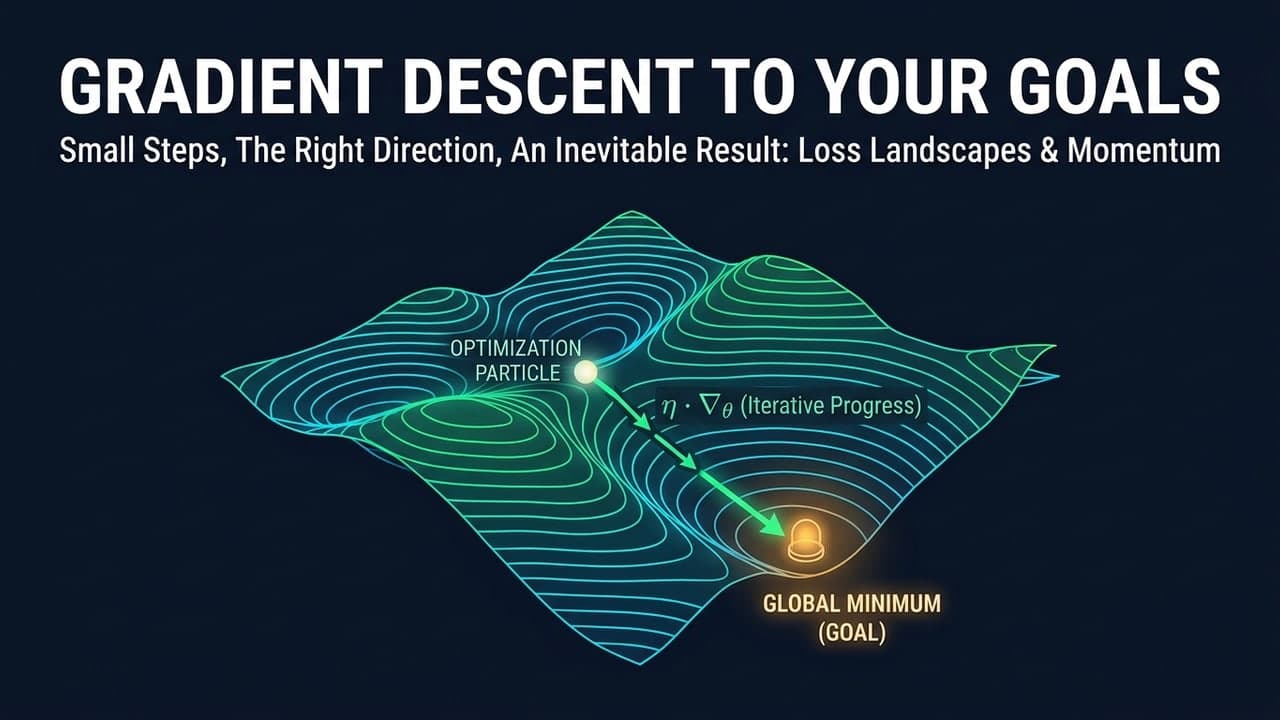
This is where the power of gradient descent goal setting becomes a transformative philosophy. Gradient descent is the foundational optimization algorithm of modern Machine Learning, powering the parameter updates of neural networks containing hundreds of billions of variables. It operates on a deceptively simple premise: you do not need to see the global minimum to find it. You only need to calculate the local slope (the gradient) of your current position and take a step in the direction of steepest descent. By translating this algorithmic blueprint into human systems, we can guarantee consistent, compounding progress that makes reaching a state of high performance a mathematical certainty.
What is a Gradient? In mathematics, a gradient is a vector that points in the direction of the greatest rate of increase of a function. By moving in the opposite direction of the gradient, we systematically find the lowest point of a valley—our optimal state.
Mapping the Mathematics of Iterative Growth
To apply gradient descent goal setting to our lives, we must first map the formal mathematical framework of continuous optimization onto human behaviors and feedback loops.
Let our parameters be represented by a vector, θ, which holds all the adjustable knobs of our daily routine. The loss function, denoted as J(θ), quantifies the distance between our current parameters and our target operating state. To ensure our model accounts for the physiological and cognitive costs of rapid change, we define J(θ) to include a regularization penalty. This penalty represents systemic friction, cognitive energy, or burnout risk. If we push our parameters to extremes too quickly, this penalty dominates, indicating that our lifestyle or operation is unsustainable. Our goal is simply to find the optimal parameter set that minimizes our loss.
In high-dimensional spaces, we cannot visualize the entire landscape of our future. However, we can compute the local gradient, which points in the direction of the greatest rate of increase of our loss. Each component of this gradient represents how a tiny change in a single habit or metric impacts our overall error. The human equivalent of a partial derivative is the feedback loop. By isolating a single variable—such as tracking the impact of sleeping 30 minutes longer on daily cognitive output—we calculate our local derivative. We do not need a perfect map of our career or health landscape; we only need to measure this local feedback and step in the opposite direction.
The variable that dictates the magnitude of our step is the Learning Rate (α). Choosing this rate is a delicate balancing act that determines whether our system converges or falls apart.
- The Over-Optimistic Step (
α ≫ 1): If we set our learning rate too high—demanding massive daily changes like transitioning from zero exercise to training three hours a day—our updates will overshoot the minimum. In optimization, this leads to divergence. The parameters oscillate wildly, burnout spikes, and the system experiences catastrophic failure, returning to a state of higher loss than where it began. - The Paralysis Step (
α → 0): Conversely, if the learning rate is too low—demanding microscopic, overly cautious changes—progress becomes virtually imperceptible. The system becomes trapped in stagnation, easily overwhelmed by environmental noise or static friction.
Modern optimizers do not use a static learning rate. Instead, they initialize with a moderately large step size to rapidly scan the landscape, and gradually scale down the step size as the system approaches its target. In practical terms, this means executing bold, exploratory shifts in our routines when we are far from our goals, and transitioning to highly disciplined, precise micro-adjustments as we near peak performance.
Traps on the Loss Landscape (And How to Escape Them)
The landscape of human optimization is rarely a smooth, convex bowl with a single, easily reachable minimum. It is highly non-convex, littered with mathematical traps that reflect our psychological and operational struggles.
A Local Minimum is a state where the local gradient is zero, but the absolute loss is still significantly higher than the global optimum. In human terms, this is the Comfort Trap or the "Good Enough" plateau. It represents a state where you are earning a mediocre salary at a comfortable job, or maintaining moderate health with minimal effort. Because any small change in your routine (such as changing careers or switching to a rigorous training program) initially increases your immediate loss (causing discomfort or stress), the gradient forces you back into the basin of the local minimum.
          Local Minimum vs. Global Minimum Landscape

             Loss J(θ)
                |
                |   /\     Comfort Trap
                |  /  \    (Local Minimum)
                | /    \___*___
                |/             \         True Optimal State
                |               \        (Global Minimum)
                |                \______*______
                +--------------------------------------- Parameters θ
To escape these local minima, machine learning models inject stochasticity (randomness) or utilize simulated annealing. In human execution, this means deliberately introducing high-variance exploration:
- Voluntary Discomfort: Intentionally disrupting your system (e.g., changing your environment, starting a side project, or learning a completely unrelated skill).
- Exploration Phases: Allocating 10% to 20% of your resources to high-risk, high-reward endeavors to discover deeper, more optimal valleys on the loss landscape.
Another common obstacle is the Saddle Point or a Flat Plateau. At a saddle point, the gradient is zero, but the parameter space slopes upward in some directions and downward in others. On a flat plateau, the gradient is extremely small across almost all dimensions. This represents those agonizing phases of life and business where you are putting in the work, but your output or progress feels completely stagnant.
To overcome these flat regions, we must adapt the classical mechanics extension of gradient descent: Momentum. Instead of updating our parameters based solely on our current gradient, we maintain a velocity vector that accumulates past gradients, weighted by a decay factor. When you hit a plateau where the local gradient drops to zero, this momentum carries you through the flat region. In human behavior, momentum is the operational baseline established by routine. When your daily motivation drops to zero, your past velocity—your automated habits—carries you forward.
Deep Comparison: The Three Archetypes of Strategic Execution
Different styles of human execution map directly to the three classic variants of Gradient Descent. Understanding these mappings reveals why certain work styles succeed while others fail.
| Optimization Strategy | Machine Learning Mechanism | Goal-Setting Counterpart | Pros | Cons |
|---|---|---|---|---|
| Batch Gradient Descent (The Perfectionist Planner) | Computes the gradient using the entire dataset before making a single update. | Planning every single detail of a 12-month goal before taking action; requiring perfect information. | Highly stable, smooth trajectory; avoids erratic behavior; works well in static environments. | Incredibly slow to update; easily paralyzed by changing environments; high risk of "analysis paralysis." |
| Stochastic Gradient Descent (The Chaotic Doer) | Computes the gradient and updates parameters using a single, randomly selected data point at each step. | High-frequency, reactionary daily pivots based on immediate feelings, the latest article, or short-term trends. | Highly dynamic; rapid feedback loops; high variance allows it to easily jump out of local minima. | Extremely noisy progress; high variance can lead to walking in circles; lacks cohesive long-term vision. |
| Mini-Batch Gradient Descent (The Agile Performer) | Computes the gradient using small, representative samples (batches) of data. | Working in short, highly focused sprints (e.g., 2-week iterations), reviewing empirical feedback, and making controlled adjustments. | The Optimal Path: Balances stability with speed; filters out daily noise while remaining highly adaptable. | Requires systematic discipline to maintain the evaluation cadence and manage batch sizes. |
This framework demonstrates that the ultimate key to gradient descent goal setting lies in adopting the Mini-Batch approach. It allows us to make consistent updates to our lives without needing perfect, long-term information, while avoiding the chaotic, circular paths of purely reactionary actions.
Real-World Algorithms of Success: Gradient Descent in Action
To validate this mathematical framework, we can analyze real-world implementations where gradient optimization was applied to habits, corporate scaling, and personal finance.
Case Study 1: The Micro-Habit Framework
James Clear’s Atomic Habits introduces the core thesis of compounding small improvements: getting 1% better every day results in a 37.78x improvement over a year, whereas getting 1% worse decays your capability to almost zero. Mathematically, this is a real-world implementation of a low-variance, constant learning rate optimization over a deterministic loss landscape.
By bounding the step size (α) to a small, manageable constant (e.g., reading 10 pages, doing 10 pushups), the optimization process remains well within the local linear approximation of our system. This prevents us from crossing the threshold into non-linear, chaotic regions where high step sizes trigger systemic failure, such as injury or exhaustion.
Case Study 2: Corporate Pivots (Slack and Instagram)
The evolution of Slack and Instagram represent corporate applications of Mini-Batch Gradient Descent with Adaptive Step Sizes.
Burbn was a complex, multi-featured check-in app. Instead of spending years perfecting this massive, bloated product, the founders analyzed a specific "mini-batch" of user interaction data. They calculated that the gradient of user engagement was heavily concentrated in a single dimension: photo sharing. They cropped out all other features, focused entirely on photo sharing, and renamed the app Instagram.
Similarly, the team at Tiny Speck was building a massively multiplayer online game called Glitch. During development, they built an internal communication tool to coordinate across offices. The game failed, but they analyzed their internal metrics (their mini-batch data) and realized the gradient of highest utility was in their communication platform. They pivoted and built Slack.
Case Study 3: Financial Debt Snowballing
The "Debt Snowball" method operates as a coordinate descent algorithm designed to reduce the dimensionality of a loss function as rapidly as possible. Rather than attempting to pay off debts based on the mathematically optimal interest rates (which requires high cognitive overhead and complex cash flows), the Debt Snowball has individuals pay off their smallest absolute balances first.
By paying off the smallest debts quickly, the number of active variables in the parameter space is reduced (e.g., from six active credit cards to three). This reduction in dimensionality simplifies the mental landscape, lowers cognitive load, and increases the psychological momentum parameter, providing the behavioral velocity necessary to tackle the remaining, larger liabilities. These case studies show that whether you are scaling a massive software platform or applying gradient descent goal setting to your daily routines, the mathematical rules remain identical.
Mathematical Implementation: Python Simulation
To demonstrate these optimization principles, the following self-contained Python script simulates how different gradient descent variants navigate a complex, non-convex loss landscape representing a human goal-seeking scenario.
"""
Goal Optimization Simulation via Gradient Descent Variants.
This script demonstrates how different optimization archetypes navigate
a complex, non-convex loss landscape representing human goal execution.
"""

import numpy as np

# Set random seed for reproducibility
np.random.seed(42)

def loss_landscape(theta):
    """
    Computes the loss J(theta) for a 2D parameter vector.
    This landscape represents a human goal-seeking scenario:
    Global Minimum is at (0, 0) with a loss of 0.
    Multiple local minima represent 'comfort traps'.
    """
    x, y = theta[0], theta[1]
    # Non-convex function with multiple local minima
    loss = x**2 + 2*y**2 - 0.3 * np.cos(3 * np.pi * x) - 0.4 * np.cos(4 * np.pi * y) + 0.7
    return loss

def compute_gradient(theta, batch_noise=0.0):
    """
    Computes the analytical gradient of the loss landscape.
    Includes an optional noise parameter to simulate stochasticity.
    """
    x, y = theta[0], theta[1]
    df_dx = 2*x + 0.3 * 3 * np.pi * np.sin(3 * np.pi * x)
    df_dy = 4*y + 0.4 * 4 * np.pi * np.sin(4 * np.pi * y)

    grad = np.array([df_dx, df_dy])

    if batch_noise > 0.0:
        noise = np.random.normal(0, batch_noise, size=grad.shape)
        grad += noise

    return grad

def run_optimizer(optimizer_type, start_theta, lr=0.05, epochs=100, beta=0.9, batch_noise=0.0):
    """
    Simulates parameter optimization over a set number of epochs.
    """
    theta = np.array(start_theta, dtype=float)
    history = [theta.copy()]
    losses = [loss_landscape(theta)]
    velocity = np.zeros_like(theta)

    for epoch in range(1, epochs + 1):
        grad = compute_gradient(theta, batch_noise=batch_noise)

        if optimizer_type == 'momentum':
            velocity = beta * velocity + lr * grad
            theta -= velocity
        else:
            theta -= lr * grad

        history.append(theta.copy())
        losses.append(loss_landscape(theta))

    return np.array(history), np.array(losses)

# Simulation Execution
start_point = [1.2, 1.2]
epochs = 50

# 1. Batch Gradient Descent (The Perfectionist Planner)
batch_history, batch_losses = run_optimizer(
    'batch', start_point, lr=0.03, epochs=epochs, batch_noise=0.0
)

# 2. Stochastic Gradient Descent (The Chaotic Doer)
sgd_history, sgd_losses = run_optimizer(
    'sgd', start_point, lr=0.03, epochs=epochs, batch_noise=0.8
)

# 3. Mini-Batch Gradient Descent (The Agile Performer)
minibatch_history, minibatch_losses = run_optimizer(
    'minibatch', start_point, lr=0.03, epochs=epochs, batch_noise=0.25
)

# 4. Gradient Descent with Momentum (The Consistent Performer)
momentum_history, momentum_losses = run_optimizer(
    'momentum', start_point, lr=0.03, epochs=epochs, beta=0.85, batch_noise=0.0
)

print("======================================================================")
print("             GRADIENT DESCENT OPTIMIZATION RESULTS                    ")
print("======================================================================")
print(f"Starting Position Parameters: {start_point}")
print(f"Starting Loss (Baseline Discrepancy): {loss_landscape(start_point):.4f}\n")

print(f"1. BATCH GRADIENT DESCENT (Perfectionist):")
print(f"   Final Loss       : {batch_losses[-1]:.6f}")
print(f"   Status           : {'STUCK IN LOCAL MINIMUM' if batch_losses[-1] > 0.1 else 'CONVERGED TO GLOBAL MINIMUM'}\n")

print(f"2. STOCHASTIC GRADIENT DESCENT (Chaotic Doer):")
print(f"   Final Loss       : {sgd_losses[-1]:.6f}")
print(f"   Status           : {'STUCK' if sgd_losses[-1] > 0.1 else 'CONVERGED WITH HIGH RESIDUAL OSCILLATION'}\n")

print(f"3. MINI-BATCH GRADIENT DESCENT (Agile Performer):")
print(f"   Final Loss       : {minibatch_losses[-1]:.6f}")
print(f"   Status           : {'STUCK' if minibatch_losses[-1] > 0.1 else 'CONVERGED STABLY TO GLOBAL MINIMUM'}\n")

print(f"4. GRADIENT DESCENT WITH MOMENTUM (Consistent Performer):")
print(f"   Final Loss       : {momentum_losses[-1]:.6f}")
print(f"   Status           : {'STUCK' if momentum_losses[-1] > 0.1 else 'CONVERGED STABLY BY SAILING PAST TRAPS'}")
print("======================================================================")
Conclusion: Trusting the Convergence
The primary lesson of continuous optimization is that our obsession with long-term foresight is mathematically misplaced. In complex, non-convex, and dynamic landscapes, attempting to map out a five-year or ten-year path in exhaustive detail is a waste of computational energy. The environment changes, local variables shift, and the initial long-range gradient computation becomes obsolete before the first step is completed.
Instead of demanding a perfect view of the summit from the base of the mountain, you must focus entirely on calculating the local gradient of the step immediately in front of you. If your feedback loops are clean (allowing you to calculate a precise gradient) and your step size is calibrated to avoid both burnout and stagnation, you do not need to see the destination to reach it. The mathematics of optimization guarantee that stepping consistently in the direction of steepest local improvement will guide you downward through the landscape.
Ultimately, gradient descent goal setting is about trading anxiety for algorithm. In numerical optimization, if a system maintains a consistent, non-zero gradient descent vector under a well-behaved learning rate schedule, convergence is not a matter of luck, inspiration, or circumstance—it is an algebraic inevitability. By treating progress as an iterative engineering problem, you strip away the emotional overhead of goal execution. You simply execute your daily parameter updates, gather local feedback, maintain behavioral momentum, and allow the mathematical laws of convergence to carry you to your goals.